Quantum Error Correction
Quantum error correction, without the mystery wall.
Quantum computers do not fail because one gate is slightly noisy. They fail because small errors keep accumulating. Quantum error correction is the idea of storing one fragile logical qubit inside a larger, redundant physical system, then repeatedly checking for error syndromes without directly measuring the logical state itself.
The alphabet first: $I, X, Y, Z$
Before talking about codes, it helps to name the objects that errors are built from. A single-qubit Pauli error lives in the set $\{I, X, Y, Z\}$:
$$ I=\begin{bmatrix}1&0\\0&1\end{bmatrix},\quad X=\begin{bmatrix}0&1\\1&0\end{bmatrix},\quad Y=\begin{bmatrix}0&-i\\i&0\end{bmatrix},\quad Z=\begin{bmatrix}1&0\\0&-1\end{bmatrix}. $$On the Bloch sphere, $X$, $Y$, and $Z$ correspond to flips around different axes. In a many-qubit system, a physical error is a tensor product $E = E_1 \otimes \cdots \otimes E_N$ with each $E_j \in \{I,X,Y,Z\}$.
Classical error correction works by adding redundancy to bits. Quantum error correction does something subtler: it spreads logical information across many physical qubits and uses carefully chosen parity-like measurements, called stabilizer checks, to detect where errors likely happened. Those stabilizer outcomes do not reveal the encoded quantum information, but they do reveal the syndrome, which is enough to guide a decoder.
The basic loop
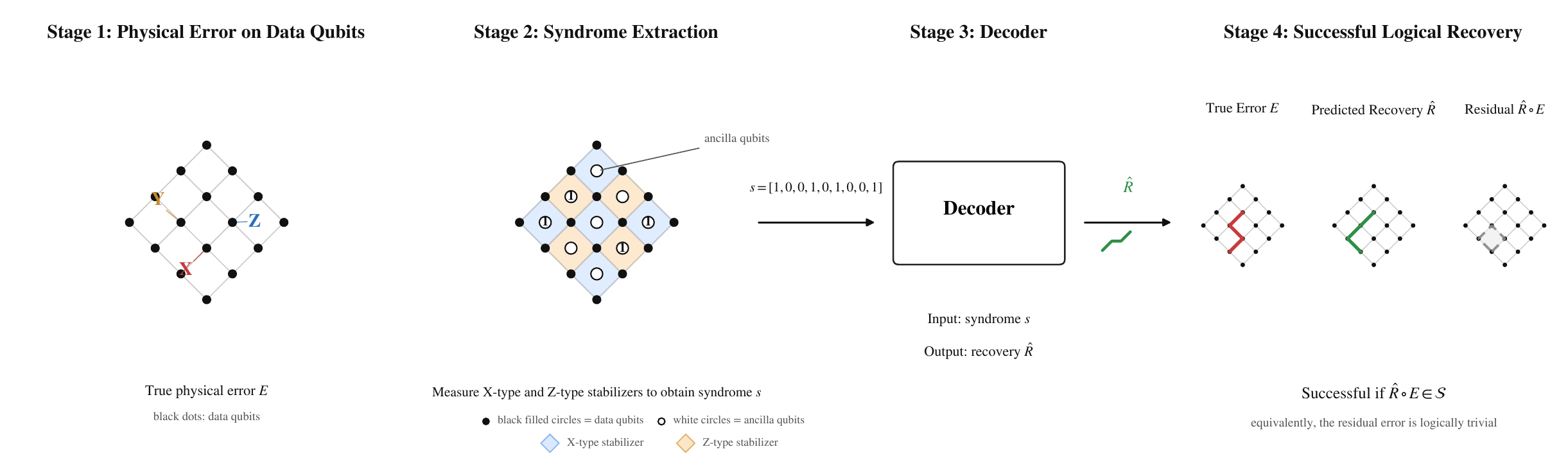
The decoder only sees syndrome information. Success means recovering the right logical state, not necessarily the exact microscopic error.
What counts as success?
A decoder does not need to guess the exact microscopic error pattern. In fact, many different physical errors are equivalent: they can have the same syndrome and act the same way on the encoded logical qubit. The real goal is to apply a correction that returns the system to the correct logical state. That is why quantum decoding is partly a pattern-recognition problem and partly a symmetry problem.
In CSS codes, it is standard to split the error into bit-flip and phase-flip parts. If $e_X$ and $e_Z$ are the binary supports of $X$ and $Z$ components, then syndrome extraction can be written as
$$ s_X = H_Z e_X \pmod 2,\qquad s_Z = H_X e_Z \pmod 2. $$This is why parity-check matrices appear so naturally in quantum decoding: they are the algebraic version of the stabilizer geometry.
The two colored check families in the figure are exactly these parity constraints. An $X$ check is one row of $H_X$, and a $Z$ check is one row of $H_Z$. In the explorer, when a colored region or highlighted constraint touches a set of qubits, that is the support of one row of the corresponding parity-check matrix.
This is also why the syndrome is so useful. It is a binary signature telling us which parity constraints were violated. The decoder does not directly observe the logical state or the full physical error pattern. It only sees which checks flipped, then uses that pattern of violated constraints to infer a recovery.
A concrete $d=3$ rotated surface code you can simulate
The rotated surface code with distance $d=3$ is the smallest example that already shows the main ingredients of the decoding problem clearly. It gives a $3 \times 3$ patch of data qubits, so there are exactly $N=9$ data qubits, $4$ $X$ checks, $4$ $Z$ checks, and one encoded logical qubit $(K=1)$.
It is convenient to number the data qubits row by row, from $1$ through $9$:
$$ \begin{matrix} 1 & 2 & 3 \\ 4 & 5 & 6 \\ 7 & 8 & 9 \end{matrix} $$With that convention, the rotated surface code can be written as the following support lists. Each set below is one row of $H_X$ or $H_Z$, written as the collection of qubits touched by that parity check.
- $X$-check supports: $\{1,2,4,5\}$, $\{5,6,8,9\}$, $\{4,7\}$, $\{3,6\}$.
- $Z$-check supports: $\{2,3,5,6\}$, $\{4,5,7,8\}$, $\{1,2\}$, $\{8,9\}$.
- Logical $X$ support: $\{1,2,3\}$.
- Logical $Z$ support: $\{1,4,7\}$.
In matrix language, that means $H_X$ has four rows and $H_Z$ has four rows. So when I write “$4$ $X$ checks” and “$4$ $Z$ checks,” I literally mean four parity constraints of each type.
These support lists already determine the syndrome rules:
- the $Z$ checks detect the $X$ component of the error,
- the $X$ checks detect the $Z$ component of the error.
If we write the current Pauli pattern as separate binary supports $e_X, e_Z \in \{0,1\}^9$, then the syndrome relations are written directly from the support lists above:
$$ s_X = H_Z e_X \pmod 2,\qquad s_Z = H_X e_Z \pmod 2. $$In practical terms, that means:
- an injected
Xor theXpart of aYerror flips nearbyZ-check syndrome bits, - an injected
Zor theZpart of aYerror flips nearbyX-check syndrome bits.
This representation is useful because it gives three things at once: the visual patch, the exact check geometry, and the algebraic objects the decoder uses.
If the decoder predicts a recovery $R$, the important question is not whether it guessed the exact physical error pattern. What matters is what remains after the recovery is applied. If the combined effect $R E$ is just the identity, or differs from it only by a stabilizer, then the encoded information is still the same and the recovery counts as a success. If $R E$ contains a nontrivial logical operator, then the logical state has changed and the recovery has failed.
That is what “same logical class” means in practice. We form the residual operator $R E$ and ask whether it is trivial up to stabilizers. If the residual is only a stabilizer, then it acts invisibly on the encoded qubit and the logical information is unchanged. If the residual still has a logical $X$, logical $Z$, or another nontrivial logical component, then the logical information has changed even if the physical qubit pattern may look locally similar.
Try the full loop on a $3 \times 3$ rotated surface code
This toy example follows the exact $d=3$ support lists above. You can inject physical Pauli errors, watch the syndrome bits flip, inspect the decoder input and predicted recovery, and then check whether the final state stays in the same logical class.
From surface codes to toric codes
The toric code takes the same stabilizer-code philosophy and wraps the lattice around periodic boundaries. Instead of a square patch with edges, imagine gluing opposite sides together until the lattice lives on a torus. That change removes physical boundaries and introduces two independent non-contractible directions. As a result, the toric code encodes two logical qubits instead of one.
That extra symmetry is not just geometric decoration. It changes the decoding problem. Surface-code decoders can use the boundary structure directly. Toric-code decoders must respect periodicity and a larger logical space.
Try the full loop on a $d=3$ toric code
This small periodic lattice has $18$ edge qubits, $8$ $X$ checks, $8$ $Z$ checks, and two logical qubits. Just like in the surface-code example, the decoder only sees syndrome bits. The difference is that the logical recovery check now has to respect two independent non-contractible directions instead of one.
Why decoders are hard
Decoding is not just about local error detection. A good decoder has to reconcile local syndrome evidence with global structure. On small examples this can be done analytically or with combinatorial algorithms. On larger systems, or with more realistic noise, it becomes natural to ask whether learned decoders can discover useful structure automatically.
That is the direction I am currently exploring: decoders that respect the Tanner-graph structure of quantum codes while still being flexible enough to model ambiguous, degenerate error patterns. This post is only a primer. I will write about the actual models, experiments, and tradeoffs later.
SAQ in one page
One useful baseline is SAQ. At a high level, it takes the observed syndrome tensor $Y_{\mathrm{syn}} \in \mathbb{R}^{M \times 2}$, turns it into binary syndrome bits, embeds those syndrome checks as tokens, and simultaneously keeps a bank of logical-class tokens. The two streams then interact through shared attention blocks.
At a high level, the flow looks like this:
$$ Y_{\mathrm{syn}} \;\rightarrow\; s \in \{0,1\}^M \;\rightarrow\; \text{syndrome tokens \& logical-class tokens} \;\rightarrow\; \text{attention blocks} \;\rightarrow\; \text{qubit logits} \;\rightarrow\; \text{CPND projection}. $$The final output is not taken directly from raw logits. A post-processing step, CPND, projects the symplectic prediction back toward parity and logical consistency. That extra step matters because it helps turn a soft prediction into a recovery that is more compatible with the code constraints.
The core SAQ idea
- Convert observed syndrome channels into binary syndrome bits and sign-valued syndrome tokens.
- Predict a logical prior over logical classes from the syndrome.
- Run shared attention blocks where syndrome tokens interact with one another, and logical tokens cross-attend to the syndrome stream.
- Aggregate syndrome information back to qubits and predict a binary symplectic error representation.
- Apply CPND projection so the final prediction better respects parity and logical consistency.
Conceptual flow
observed syndrome → syndrome bits
→ logical prior + syndrome tokens
→ shared attention
→ qubit logits
→ CPND projection
This is the high-level idea I want to emphasize here: what information SAQ uses, how that information is organized, and why a projection step matters at the end.
Why I still care about better decoders
A natural question comes up once you read the recent literature: if a baseline such as SAQ is already close to the maximum-likelihood (ML) threshold, is there really much room left for a new decoder to improve? The short answer is yes, but the room is subtler than “move the threshold dramatically upward.”
In quantum error correction, the word threshold usually refers to a crossover in physical error rate. Roughly speaking, below that crossover, increasing the code size helps drive the logical error rate down; above it, making the code larger stops helping. That is different from the classical coding question “for this fixed channel, what is the best BER I can possibly achieve?” So when someone says a decoder is close to the ML threshold, they are usually saying it already gets close to the best known crossover point, not that every finite-size logical error curve is already optimal.
That distinction matters. Even if two decoders have very similar thresholds, one of them can still have noticeably better logical error rates at a fixed code size and a fixed physical noise level. In practice, that is often the regime people care about most. Real devices do not operate at infinite code size. They operate at one concrete distance, under one concrete noise model, with one concrete latency budget.
That is exactly where I think MDM-style decoders can still be interesting. A structured diffusion decoder is not trying to beat the laws of the code family. It is trying to use the syndrome geometry more effectively at finite size, especially in regimes where degeneracy, ambiguity, and global consistency all matter at once. In other words, even if SAQ is already near the ML threshold for some setting, there may still be room to improve the actual logical error rate for physical error rates below that threshold.
So the question I care about is not only “can a new decoder shift the threshold?” but also: for a fixed physical error rate below threshold, can it produce a lower logical error rate, a more robust recovery, or a better tradeoff between quality and computation? For toric codes in particular, where logical ambiguity and periodic structure are both strong, that still seems like a very meaningful target.
What I want to explain next
The natural follow-up is to compare why SAQ and diffusion-style decoders behave differently on surface and toric codes, especially when logical ambiguity and post-processing start to dominate.
Direct link: /blog/quantum-ecc-primer/